Optical Telescopes, Radio and X: main principles and differences – Part TWO – Radio telescopes
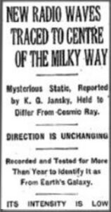
Radio astronomy is a relatively young science compared to optical astronomy. It found its early developments in the 1930s, over 300 years after the first observations in the visible spectrum. It was Karl Jansky, a researcher at Bell Telephone Laboratories in 1931, who, using an array of antennas over 30 meters in length, recorded radiation with a wavelength λ = 14.6 meters (20.5 MHz), demonstrating that it must have an extraterrestrial origin. The faint but continuous “hiss” detected by Jansky’s antenna would rise and set on a daily basis, giving the impression of coming from outside our planet. Although initially it seemed to be caused by solar radio emissions, by more precisely calculating the celestial coordinates of its origin, it was understood that this signal came from the constellation Sagittarius, i.e., from the center of our galaxy. A few years later, engineer Grote Reber published the results of his observations with the first parabolic radio telescope at λ = 1.87 meters in an astrophysics journal, showing the first radio survey of a galaxy. By further improving radar technologies developed during World War II, radio observations made significant progress, and the scientific-astronomical community began to take an interest in this field.
A radio telescope consists of an antenna composed of a reflective surface that collects radiation and a receiver that detects, filters, and amplifies the collected radiation. Since radio astronomy works at wavelengths ranging from about 0.5 mm (600 GHz) to 20 meters (15 MHz), the structure of radio telescopes is less restrictive than optical telescopes. The antennas can be large parabolic dishes or filamentary arrays that extend for many meters. To have adequate reception sensitivity, the dimensions of the structure’s components need only be smaller than or equal to λ/4.
Radioastronomical signals do not exhibit any modulation; they appear as an incoherent signal with a continuous spectrum radiated simultaneously across all frequencies, essentially as noise.
Antennae
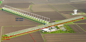
The linear antenna, composed of metallic wires, is the simplest type of construction and is used for wavelengths λ > 1 meter. Generally, the structure consists of multiple wires with different shapes. It is organized so that the arrays form a dipole. Through it, it is possible to detect the electromagnetic radiation from the source and transform it into an electrical signal. A typical example is the Northern Cross Antenna in Medicina (Bologna), which consists of two series of antennas: one oriented from East to West and the other from North to South. The first is a single large antenna that is 546 meters long and 35 meters wide, consisting of 1536 dipoles, and the second is a linear array consisting of 64 antennas placed 10 meters apart from each other.
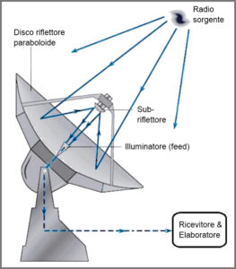
For wavelengths λ < 1 meter, single paraboloids are used, similar to those used in optical telescopes, but always made of metal mesh, or more complex configurations like multi-dish setups (interferometers, see § 3.4). The primary reflector (made of aluminum) is a parabolic surface that focuses the incident radiation onto the sub-reflector, which is the secondary hyperbolic reflector, which in turn reflects the incident waves toward the feed antennas (feeds). The sub-reflector can also be rotated to direct the radiation to different feeds (of different frequencies). The receiver then converts the detected waves into electrical voltage, which is subsequently processed and visualized using appropriate analysis software.
Just like in optical telescopes, the resolution of an instrument in radio astronomy is directly proportional to the wavelength λ: Θ = 1.22 λ/D, where D is the diameter of the telescope or the maximum distance between telescopes in an array. However, when working with wavelengths ranging from millimeters to a few meters, it’s evident that, for the same diameter, a radio telescope has a significantly lower resolution compared to an optical telescope that operates at wavelengths on the order of micrometers.
Antenna performance parameters
An antenna is typically described by several parameters that define its performance. The main ones are efficiency and the shape of the power pattern beam.
Aperture efficiency describes the ratio between the effective aperture, Ae, and the geometric aperture, Ag (which is proportional to D2 – the actual collecting area of the antenna). This measures how much power is extracted by the ideal antenna from incident radiation with a certain power density. Efficiency, denoted as η, is therefore the ratio between this quantity and the geometric aperture, considering the antenna’s shape.
η = Ae / Ag
It is a measure of the deviation from the ideal case in which the absence of signal losses would result in an effective area equal to the geometric area of the antenna: η is always < 1, typically ranging from 0.5 to 0.7, and dependent on frequency. Aperture efficiency is thus influenced by the quality of the mirror’s surface, such as gaps between panels or deviations from the theoretical shape (gravity, wind, and thermal expansions contribute to distorting the ideal structure), as well as blockage of the aperture caused by supports, receivers, and sub-reflectors that obscure part of the mirror.
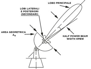
The beam, also called the “power pattern,” is a measure of the received power as a function of angular distance from the instrument’s axis. The radiation diagram of the antenna-illuminator combination (Power Pattern) is the three-dimensional representation of its gain. Often, antennas do not have a symmetrical radiation pattern but instead have a central lobe and secondary side lobes that limit their quality and can also generate interference. To achieve optimal reception, the diameter of the parabola should correspond to the maximum width of the illuminator’s radiation lobe.
The resolution of a radio telescope is called the “Half Power Beam Width” (HPBW) and represents the width of the main lobe at half its peak height. It can be approximated as HPBW ≃ λ/D. To achieve high resolutions, one needs to operate at higher frequencies and use very wide lobes, which in turn requires very large antennas.
Receivers
Receivers in radio astronomy are used to detect and measure the signal collected by the antenna, and they consist of various components. First, the feed (illuminator) collects the electric field component of the electromagnetic wave and converts it into a voltage. It typically has a horn-shaped design to match the wavelengths of microwaves, with dimensions comparable to λ, and is placed at the center of the parabola where the energy is concentrated. For large radio telescopes, the illuminator consists of an array of horn feeds (for different frequencies) maintained at low temperatures.
The receivers used in radio astronomy are mostly of the superheterodyne type, a term that identifies receivers converting the incoming signal into a new signal that contains the same information but at a lower frequency. The receiver can be divided into two blocks:
- Frontend: This consists of a low-noise amplifier, a filter for higher and lower frequencies (bandpass filter), and a mixer that combines the radio signal with a monochromatic signal, much stronger than the original, generated by a local oscillator at a frequency close to that of the original signal (to achieve high stability).
- Backend: This includes another bandpass filter. Since the radioastronomical signal appears as a weak, rapidly varying, random voltage, a simple measurement of its mean value over time would yield a null result. For this reason, a device is used that not only measures the signal’s amplitude but also its square (Square Law Detector – SQLD). Finally, the signal output from the detector (proportional to the square of the original signal) is sent to an integrator, which averages it over a specific time interval to remove noise introduced by the electronics.
Noise is primarily caused by the receiver, and to obtain good results in an observation, it is necessary to have a high signal-to-noise ratio. To reduce noise, it is useful to have long integration times, which means observing the same source for an extended period and having a good Half Power Beam Width (HPBW), as seen earlier, depends on the ratio between λ and D, so the dimensions of the primary mirror should be as large as possible. There are also other sources of noise, such as sources outside the Solar System (cosmic noise) or within it (solar noise).
In all these cases, of course, the noise depends on the pointing direction of the antenna and increases in the vicinity of the galactic plane, while away from it, it is limited to the cosmic background radiation. Even terrestrial sources can be a source of noise. When radio signals pass through the various layers of the atmosphere, they can undergo attenuation due to molecular absorption, rain, and electrical discharges. Therefore, the atmosphere can be seen as an additional source of noise.
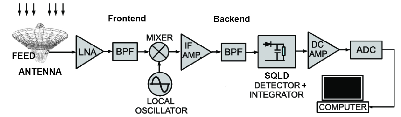
Radiotelescope scheme
Interferometry
Since the resolving power of a telescope depends on its diameter and the wavelength of the incident radiation, achieving excellent angular resolutions with radio telescopes is very challenging because it would require antenna diameters of hundreds or thousands of meters to achieve resolutions comparable to optical telescopes. Building such large radio telescopes would pose problems related to costs and, more importantly, structural integrity. The world’s largest radio telescope, FAST in China, has a diameter of 500 meters but is constructed in a natural karst depression to support the dish, making it a non-steerable, transit telescope that can only observe sources that pass near the zenith.
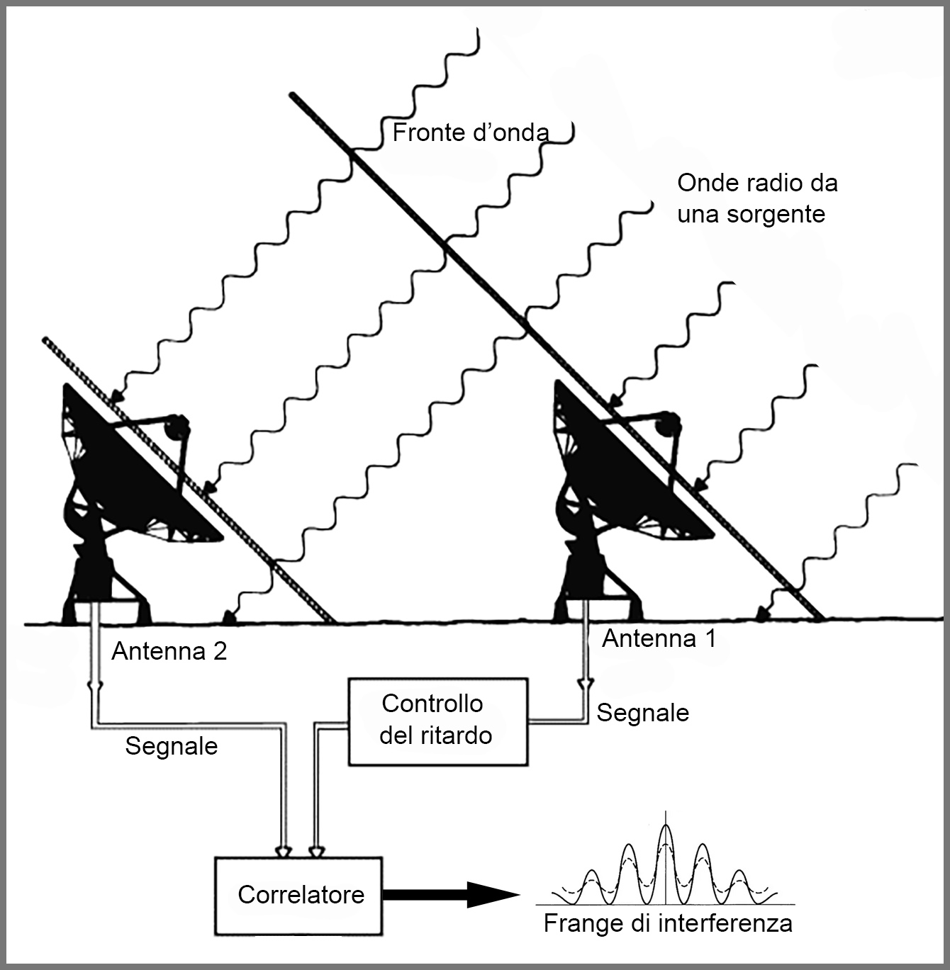
Hence, radio astronomers resort to interferometry. An interferometer is a system of two or more antennas connected to each other, observing the same source simultaneously. They are all connected to a single receiver, and their separation (D) is called the baseline. The resolution of the interferometer is equal to that of a single antenna with a linear size of D. Naturally, the received power is proportional to the sum of the surface areas of the individual antennas, meaning its sensitivity is proportional to the number of antennas used, S = ND2 (with D being the antenna diameter). Interferometry is based on the concept of interference: the principle of superposition expresses the fact that the resulting wave from the combination of separate waves (interference) has properties related to those of the original states of the waves themselves. In particular, when two waves with the same frequency combine, the resulting wave depends on the phase difference between the two waves: in-phase waves undergo constructive interference, while out-of-phase waves undergo destructive interference.
In the hardware of an interferometric system, the correlator is very important: the signals from each antenna are sent to the digital correlator, which, based on the Fourier transform, performs the necessary calculations for correlating the various signals and outputs the visibility functions for each baseline of the array antennas.
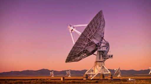
Among the most important interferometers are ALMA (Atacama Large Millimeter/submillimeter Array) in Chile, consisting of 66 antennas at distances of up to 16 kilometers, the VLA (Very Large Array) in New Mexico, USA, consisting of 27 antennas arranged along three arms, each 21 kilometers long, in a Y-shape, and VLBI (Very Long Baseline Interferometry), which has no connections between antennas and operates on a global scale. Digitized data are typically recorded for each of the telescopes on hard drives, then transferred via the Internet, with a highly precise atomic clock-generated time stamp. The signal is later correlated through supercomputers at a central data processing facility.